
Anti-Aliasing.com
Sampling Functions
Aliasing effects can be analyzed using the Nyquist frequency and the Nyquist–Shannon sampling theorem.
Sampling Functions
Nyquist Frequency: When displaying a repetitive pattern, the Nyquist frequency defines the
maximum allowable frequency before aliasing occurs.
Definitions from Wikipedia
Nyquist frequency: https://en.wikipedia.org/wiki/Nyquist_frequency
Nyquist Rate: https://en.wikipedia.org/wiki/Nyquist_rate
Nyquist–Shannon sampling theorem:
https://en.wikipedia.org/wiki/Nyquist%e2%80%93Shannon_sampling_theorem
Book References
There is a great book reference about analysis of signal aliasing and jaggies by:
Blinn, James F.: Jim Blinn’s Corner: Dirty Pixels,
Morgan Kaufmann Publishers, Inc., 1998, ISBN 1-55860-455-3
Chapter 2: ‘What We Need Around Here is More Aliasing’
Chapter 8: ‘The Wonderful World of Video’
Chapter 3: ‘Return of the Jaggy’
Chapter 13: ‘ NTSC: Nice Technology, Super Color’
Spatial Domain and Frequency Domain
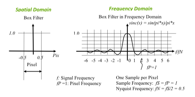
When taking samples within a pixel and all samples have the same weight, the sampling
window in Spatial Domain is a Square Window, or Box Filter.
In the frequency domain, the frequency response for a Box Filter is a sinc() function.
Refer to Wikipedia and Figure 1:
Sampling Function sinc(): https://en.wikipedia.org/wiki/Sinc_function
Aliasing when Signal Frequency Greater than Nyquist Frequency
When the signal frequency is greater than the Nyquist Frequency, this results in signal frequency aliasing. In the frequency domain, the frequency response for a Box Filter is a sinc() function. The Refer to Figures 2 & 3.
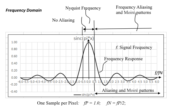
This frequency response indicates that when sampling a sine wave of frequency fP=1.0, there should be 2 samples per pixel to prevent aliasing. When 2 samples of the sine function are taking inside of the pixel, the average for the pixel will be 0.0, which prevents aliasing.
Anti-Aliasing Acts as Low pass Filter.
In the previous section, the Nyquist frequency for a box filter and one Sample per Pixel was evaluated as:
Pixel Frequency fP = 1.0;
Nyquist Frequency for 1 Sample Point: fN = fP/2;
Incremental Steps with ABAA 4 & 8
With ABAA and N subpixel areas, the pixel is divided into N incremental steps, independent of edge angle. This corresponds to a lowpass filter, since the contributions inside of the pixel are averaged. This lowpass filter extends the aliasing frequency by a factor N.
The Nyquist frequency for ABAA 4 becomes: fN(ABAA4) = 4*fP/2 = 2fP
The Nyquist frequency for ABAA 4 becomes: fN(ABAA4) = 8*fP/2 = 4fP;
With ABAA, the incremental areas are constant, regardless of edge orientation. This is important to prevent narrow face breakup.
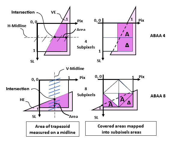
Examples with ABAA4 & 8
In Figure 4, there are 2 examples of a triangle edge intersecting a pixel. The intersection of the triangle edge with the midline is where the covered area is measured. On each midline, the increments across the pixel are constant for ABAA4 (=1/4) and for ABAA8 (=1/8).
ABAA 4
In this example with ABAA 4, the intersection is at 2/4.
The area is measured on the right side as: 2/4=1/2.
For narrower faces, potential breakup of a face 1/4 pixel wide would have an intensity delta reduced by 1/4.
ABAA 8
For ABAA 8, the intersection is at 5/8. The area is measured on the lower side as: 3/8.
For narrower faces, potential breakup of a face 1/8 pixel wide would have an intensity delta reduced by1/8.
Narrow Face Breakup with MSAA
The purpose of point sampling approach is to convert analog signals into digital signals. An important condition is that the analog signal should be continuous. This is true for the area and the contour of faces that are wider than 2 pixels. This is not true for faces narrower than 1 pixel wide. Note that for triangle faces 2 pixels wide, the average triangle width is 1 pixel wide.
Sample Gaps and Narrow Face Breakup
When faces get narrower than 1 pixel wide, the gap between 2 edges crossing subpixel sample points can became wider than the face width. Also, the contours on both sides of a face can become too close to each other. This will result in narrow face breakup.
For single sample points, the distance between sample points is 1 pixel wide. For N subpixel sample points, the distance between transitions as edges cross the sample points depends on the triangle edge slopes.
MSAA with HE and VE
In Figure 5, there are 4 examples for MSAA with edges at 0 degrees (HE or VE) and edges at ~30 degrees. The two examples in the first row are for MSAA 4, while the examples in the second row are for MSAA 8. For MSAA 8, the example uses a modified solution to the eight Queens (Q) puzzle.
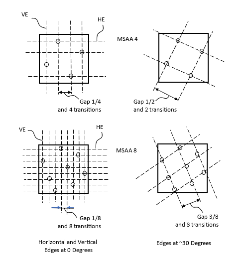
MSAA4 with Edges at 0 Degrees
These examples use sample points selected according to the ‘N rooks puzzle’, with N=4 and N=8. This represents the best cases for HEs and VEs with edge slopes at 0 degrees, and the worst cases for edges slopes at roughly 30 degrees.
In the two left examples, the gaps between edges transitions at 0 degrees are only 1 subpixel wide, that is 1/4 for MSAA4 and 1/8 for MSAA8. As an HE, or VE, moves across the pixel area, the transition from not covered to completely covered changes uniformly from 0.0 to 1.0.
the selected edges are HE of VE with angle at 0 degrees. The gaps between sample points are only 1 subpixel wide
For MSAA 4 (edges at 0 degrees): fN(MSAA4-0) = 4*fP/2 = 2fP
For MSAA 8 (edges at 0 degrees): fN(MSAA8-0) = 8*fP/2 = 4fP
MSAA with edges at 30 degrees
In the two left examples, the worst case for edges at (roughly) 30 degrees and the resulting large gaps between edges are identified. Because of aligned sample points, the gaps between transition have grown to 1/2 for MSAA4 and 3/8 for MSAA8.
For MSAA 4 (edges at 30 degrees): fN(MSAA4-30) = 2 fP/2 = fP
For MSAA 8 (edges at 30 degrees): fN(MSAA8-30) = 4/3 fP.
In these examples at 30 degrees, the larger gaps can cause narrow face breakup for faces narrower than 1/2 pixel wide. At the same time, the gaps between adjacent edges result in edges lining up with several sample points, which amplifies the intensity delta and makes the gaps more noticeable.
Note: In this case, the gap for MSAA8 is only 33% better than MSAA4. This is only a minor improvement, considering the 100% increase in computing time.
In the worst case, with MSAA4, there are only 2 samples per pixel, with twice the amplitude.
In the worst case, with MSAA8, there are only 3 samples per pixel, with 3 times the amplitude.
When considering the narrow face breakup with MSAA 8, the result is only slightly better than MSAA 4.
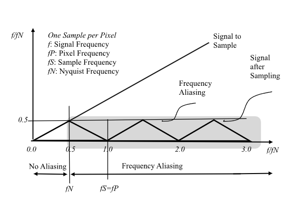
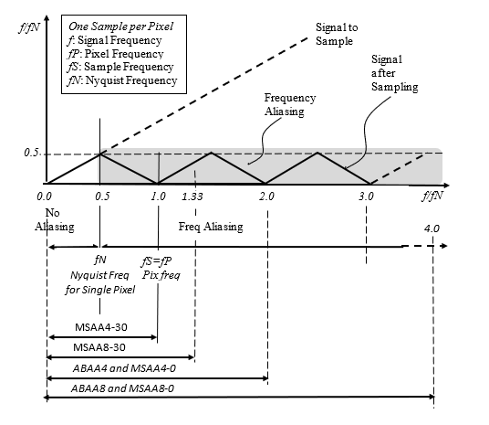
Comparison between ABAA and MSAA
In Figure 6, the low pass effect of anti-aliasing is shown for ABAA and MSAA. The shaded area in the figure shows the region of aliased frequencies that result from single point sampling. When using anti-aliasing with MSAA and ABAA, the Nyquist frequency is extended. For each of the methods (and angles for MSAA), an arrow shows how far the low-pass extend the Nyquist frequency.
Pixel Frequency fP = 1.0;
Nyquist freq. for single sample point: fN (Single Sample Point) = fP/2;
For a sine wave of frequency fP, in order to prevent aliasing, there should be at least 2 sample points per pixel. That is: 2 horizontally and 2 vertically, like MSAA 4.
Nyquist Frequencies with anti-aliasing for ABAA
ABAA 4: fN(ABAA4) = 4*fP/2 = 2fP;
ABAA 8: fN(ABAA8) = 8*fP/2 = 4fP;
Nyquist Frequencies with anti-aliasing for MSAA
MSAA 4: fN(MSAA4-0) = 2 fP;
MSAA 4: fN(MSAA4-30) = fP;
MSAA 8: fN(MSAA8-0) = 4 fP;
MSAA 8: fN(MSAA8-30) = 4/3 fP; (only 33% better than MSAA4)
Conclusion
Although MSAA is as good as ABAA for edges are 0 degrees angle, the worst case at 30 degrees should be used for evaluation, because it is the only way to remove narrow face break up.
From this comparison between MSAA4 and MSAA8, it turns out that MSAA4 is almost as good as MSAA8, at half the price.
As a result from this analysis, besides being the fastest approach, ABAA is definitely superior to MSAA. ABAA should be used for future product developments.