ABAA vs MSAA Simulation

Comparison of Anti-Aliasing Techniques

While most of the current approaches to anti-aliasing rely on ‘point-sampling, ABAA uses a new approach that relies in area-sampling. In this section, 3 types of solutions are compared:
– Compute the image with point-sampling, followed by image post processing.
– Compute several images with point sampling, followed by averaging the images.
– Compute the image directly with anti-aliasing, using area-based sampling.

First, the point sampling methods are compared.
Then, simulated images for ABAA and MSAA are compared. 

Comparison of Point Sampling Methods  

In this section, several anti-aliasing methods are compared.

In Figure 1, there are comparisons between five anti-aliasing methods that rely on point sampling. It looks like the images in the top row have a resolution of 80×80 pixels and the lines have a 1.0-pixel width. The images in the bottom row have a resolution of 40×40 pixels and the lines have a 0.5-pixel width. In the first 3 examples, the images are computed with single point sampling, followed with postprocessing. In the last 2 examples, the images are computed with MSAA4 and MSAA8.

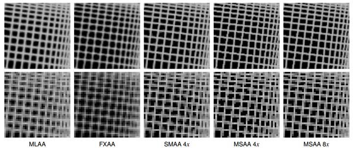
Figure 1 Comparison of Anti-Aliasing Techniques,
from https://vr.arvilab.com/blog/anti-aliasing

Note that there are many “narrow face breakups” in the FXAA image in the 2^nd row. The lines of width 0.5-pixel cause the links to breakup. Also, the line crossings are blown-up (or blurred) in the first row.

It is unfortunate that images rendered with single point-sampling (without processing) were not available. This would have given some hints about the effectiveness of these approaches. The image rendered with FXAA is probably the closest to the point sampling image where the pixels with high contrast have been blurred.

In Figure 2, there is an attempt to show what the same image would look like with single point sampling. This image of size 24×16 pixels corresponds to 1/4 of the images in the 2^nd row. The line width is 1/2 pixel.

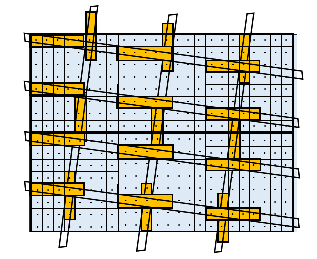
Figure 2 Example of Narrow Faces of Width ½ Pixel using 1 Sample Point

In these examples, MSAA 4x and 8x produce the best images, but at the cost of increased processing time (lower frame rate). MSAA should produce the best results for near horizontal and near vertical lines. But the results can vary for different line angles. Notice the broken lines (hardly noticeable) on the top left corner of the last 2 images in the 2^nd row. Results with ABAA will be as good or better, without the speed penalty.

These images have been produced with existing systems. Since ABAA is new, there are no comparable images from existing systems. For this reason, ABAA are compared with MSAA using simulation.

ABAA vs MSAA Simulation

With ABAA, only a single image needs to be computed, compared with 4 images with MSAA4 and 8 images with MSAA8. Although no similar images are available for ABAA 4 & 8, some the following results can be expected.

In the second row of images, the face width is 1/2 pixel wide. ABAA4 can handle line width 1/4 pixel, which is 2 times narrower. ABAA8 can handle line width 1/8 pixel, which is 4 times narrower. The same images produced with ABAA will be better than images from MSAA.

Comparison of ABAA vs MSAA with Fans of Triangles

The advantage of ABAA over MSAA is more noticeable for faces narrower than ½ pixel wide. Several cases are simulated with ABAA and MSAA in separate figures below. Each test case consists of 8 narrow triangles of height 8 pixels and base 1 pixel. Each triangle can be divided into 8 slices 1 pixel thick. From these 8 slices, there are 8 cases of narrow width between 1/16 to 15/16 pixel. It will be shown that ABAA produces the best images.

In the first figure, the same test with a fan of 8 thin triangles is processed with both ABAA4 and MSAA4. The same test will be also simulated with ABAA8 and MSAA8,

Then the result of four similar test cases consisting of 8 thin triangles with different orientation are simulated and summarized.  The first case is repeated, followed by 3 other test cases. These 4 test cases are first simulated with ABAA4 and MSAA4, then simulated with ABAA8 and MSAA8.

When printed, images with gray shades can be easier to evaluate at first. But, because of the limitation of the printing process, the results can be inconclusive. Instead of gray shades, in each triangle the covered Subpixels are identified with a face identifier, from, ‘a’ to ‘h’. The results consisting of the number of covered subpixels per 1/8-pixel slices are tabulated in summary tables, beside the fans. In the summary tables, the covered Subpixels inside slices of the thin triangles should show with incremental counts per Pixel or per Scanline. So, it should be easy to evaluate and compare the ABAA vs MSAA approaches.

Four Test Cases

Four test cases have been simulated. For the 1^st test case, the detailed results for ABAA and MSAA are shown inside of 8×8 pixel spans. For the other 3 cases, the results are shown only in summary tables.

Test Cases Consisting Fans of 8 Narrow Triangles (Tri-Fans)

For the simulation, each pixel is processed with a resolution of 4 & 8 Subpixels, using ABAA and MSAA. Each test case image consists of 8 narrow triangles organized as a fan within a 90 degrees angle. Each triangle is defined by 3 edges within an 8×8 Pixel Span.

In each fan, there are 2 sets of 4 triangles.

• There are 4 ‘vertical’ triangles (a, b, c & d) within 45 degrees of vertical axis (VE), 8 SL long.
• There are 4 ‘horizontal’ triangles (e, f, g & h) within 45 degrees of horizontal axis (HE), 8 pixels long.

The triangle bases are 1 Pixel wide.

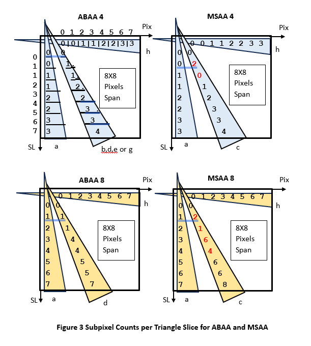
The expected result is that the number of covered subpixels corresponds to the area covered by the triangle inside of each pixel row for HE, or column for VE.

Figure 3 is shown to illustrate how to evaluate the results of the simulation.  For ABAA, all cases match the expected result.  For MSAA, only triangles ‘a’ and ‘h’ match the expected result.

For triangles in ‘b’ to ‘g’, c is selected to show a failed case for MSAA4.

Each 8×1 triangle can be divided into 8 slices, 1 pixel thick. The averages of the slice widths are:

  1/16, 3/16, 5/16, 7/16, 9/16, 11/16, 13/16, 15/16.

For 4 subpixels, this corresponds to: 0, 0, 1, 1, 2, 2, 3, 3 subpixels

For 8 subpixels this corresponds to: 0, 1, 2, 3, 4, 5, 6, 7 subpixels

Simulation with 4 Subpixels: ABAA4 is Better than MSAA4

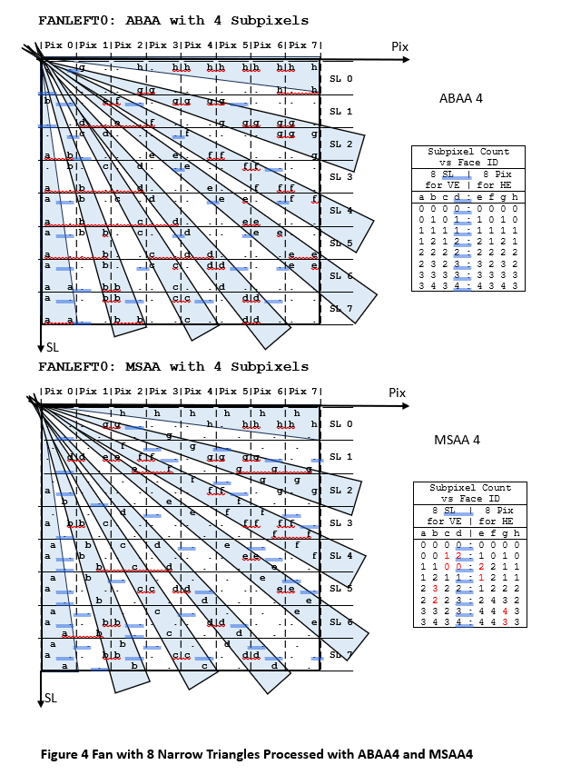
In Figure 4, the 1^st test case is processed with 4 subpixels, using ABAA4 and MSAA4.  Because of the limitation of the printing process, the comparison between these 2 methods uses subpixel counts per pixel instead of gray shades. The test images consist of 8 narrow triangles of size 1×8 pixels (base=1 and height=8) inside of an array (span) of 8×8 pixels.

Note that in the figure, the triangles are drawn slightly larger than their actual size, so that they contain all the drawn subpixels. Actually, in the program simulation the bases of the narrow triangles have a with=1 and line up exactly with the pixel boundaries at the bottom and on the right side of the 8×8 span. For example, the right edge of triangle ‘a’, intersects the 9 SL boundaries from top at 0/8 to bottom at 8/8 pixels, exactly.

Using a C/C++ simulation, the same set of triangles is processed first with ABAA4 (top span), then with MSAA4 (bottom span). In each triangle inside of the span, the covered subpixels are identified by the face ID (‘a’ to ‘h’). The subpixels not covered are shown with a dot.

Using the result from the simulation, the subpixel counts have been tabulated in small summary tables beside the simulated fans for ABAA4 and MSAA4. In the summary tables, on the right side of each span, the subpixel area counts per pixel-row or SL-column are shown. For the 4 near-vertical faces (‘a’ to ‘d’, with VEs), the subpixel counts are shown for the 8 SL-rows. For the 4 near-horizontal faces (‘e’ to ‘h’, with HEs), the subpixel counts are shown for 8 pixel-columns.

As can be seen, the subpixel counts for ABAA4 are consistent. They are independent of edge angles and increment uniformly from top to bottom of the narrow triangles. This is not so for MSAA4.

In most cases with ABAA4, the increments are either:
0, 0, 1, 1, 2, 2, 3, 3, or
0, 1, 1, 2, 2, 3, 3, 4

With MSAA4 this is only true for near vertical edges (VE) and near horizontal edges (HE) orientations. This is because the subpixels are positioned according to a solution to the 8 queens-puzzle. For other edge orientations, the increments are not smooth. There are some steps with decrements (reverse count in red in the summary tables). Also, for faces c and d, with MSAA4 there is “narrow face breakup” at width of 1 subpixel (1/4 pixel).

From this example, it is clear that ABAA4 is superior to MSAA4: faster, more accurate and better images.

Comparison between Figure 1 and Figure 4

In 1^st row of figure 1, each square image consists of 80×80 pixels. The width of the lines is 1 pixel.

In the 2nd row of figure 1, each square image consists of 40×40 pixels. The width of the lines is 1/2 pixel

In Figure 4, when compared to the 2^nd row of figure 1, the size of each pixel is magnified 12 times.

With the ABAA4 rendition, we can clearly distinguish line widths between 3/16 and 5/16 (~1/4) pixel.

With MSAA, there is “narrow face breakup” (0 subpixels), at 5/16 pixels width.

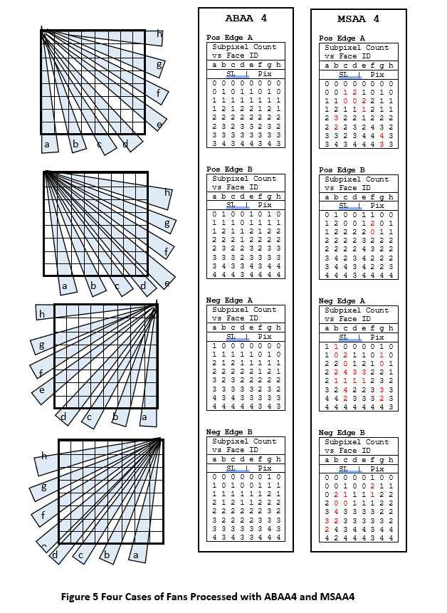
Four Fan-Cases of 8 Narrow Triangles, with 4 Subpixels

For the 1^st test case, the covered subpixels were shown in Figure 4. For the 3 other fan tests, the results are only shown in summary tables in Figure 5.

In each of these four examples, 8 narrow triangles are displayed within an 8×8 Pixel Span, spreading over an angle of Pi/2 (90 degrees). For ABAA4 and MSAA, the results are shown in 4 summary tables each. For each of the 8 triangles, the 8 covered subpixel counts are displayed in one column of the summary table.

The 8 subpixel counts for ABAA4 are incremented between 0 and 4, using half steps.
This is not always so for MSAA4. In a few cases, there are ‘narrow face breakup” at width 5/16 (3^rd row). There are also decrements (highlighted in red, in the summary tables).

From these examples, it is clear that ABAA4 is much better than MSAA4.

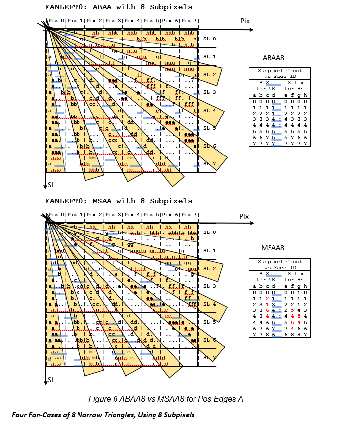
Simulation: ABAA 8 is Better than MSAA 8

In Figure 6, the same 1^st test case is now processed with 8 subpixels, using ABAA8 and MSAA8. Similar results are obtained when comparing ABAA8 with MSAA8.

Since the triangle tops are 0.0 Pixel wide and the bottoms are 1.0 Pixel wide, it is expected that the number of subpixels per pixel from top to bottom of triangles will be incremented in 8 uniform steps.  The increment for each step should be 1/8 pixel (or 1 subpixel) each. With ABAA8 most widths are rendered in steps of 1/8 pixel.

Results for ABAA8

For ABAA, in most cases, the increments are:
0, 1, 2, 3, 4, 5, 6, 7, or
1, 2, 3, 4, 5, 6, 7, 8

Results for MSAA8

Some Good: For MSAA, the increments are similar to ABAA when the triangles edges are near Vertical (face a) or near Horizontal (face h). This is because the Subpixels are positioned according to the 8 Queen algorithm.

Some Bad: For other orientations, the increments are not constant, with many increments of 2. There is also ‘hesitation’, when there are some steps with decrement (highlighted in red, in the summary tables).

These examples are shown in more details in the books.

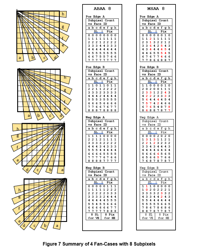
In Figure 7, four fan-cases have been simulated. In each of these four examples, 8 narrow triangles are displayed within an 8×8 Pixel Span, spreading over an angle of Pi/2 (90 degrees).
For ABAA8 the results are shown in 4 summary tables.
For MSAA8 the results are shown in 4 summary tables.
For each of the 8 triangles, the 8 covered subpixel counts are displayed in one column of the summary table. The 8 subpixel counts for ABAA8 are incremented from 0 to 7 or 1 to 8. This is not so for MSAA8 (highlighted in red, in the summary tables).

I should be noted that there are no apparent “narrow face breakup” (beside hesitation) in these examples for MSAA8.

It is directly apparent that ABAA8 is superior to MSAA8.

Conclusion

Since ABAA4 and ABAA8 require only one frame processing and no post processing, they are as fast a 1 sample point per pixel. ABAA is the fastest approach and is ideal for RT CGI. Because of its efficiency, simplicity and lower cost, the ABAA solution should be widely accepted for new product development.

In a few words:

ABAA is the Affordable & Best Anti-Aliasing Solution